A Guided Tour: What 6.7 Million Samples Can Tell You

Seven views of the Interactive Explorer, and the questions each one answers

The Interactive Explorer covers ~6.7 million physical samples — rock cores, potsherds, tissue vouchers, museum specimens — about 6 million of them on one globe, running entirely in your browser with no server behind it. This tour walks through seven views of it, each answering a question about the data. Most steps are live links — click one and the Explorer opens at the position, search, and zoom being described (the URL carries that state; a couple of steps ask you to click one control yourself, where the URL doesn’t reach).

A few steps also include a small “the number behind the view” code cell that computes what you’re seeing, live, from the same public data files the Explorer itself reads. Unfold the code to see how — and to take your first step from viewing the data to querying it.

(This page replaces an earlier “Zenodo deep-dive analysis” tutorial from the 2025 migration era; the browser-analysis techniques it demonstrated are now the Explorer’s own architecture. For how that works, see the pointers at the end.)

duckdb = import("https://cdn.jsdelivr.net/npm/@duckdb/duckdb-wasm@1.28.0/+esm")
Plot = import("https://cdn.jsdelivr.net/npm/@observablehq/plot@0.6/+esm")

db = {
  const JSDELIVR_BUNDLES = duckdb.getJsDelivrBundles();
  const bundle = await duckdb.selectBundle(JSDELIVR_BUNDLES);
  const worker_url = URL.createObjectURL(
    new Blob([`importScripts("${bundle.mainWorker}");`], {type: 'text/javascript'})
  );
  const worker = new Worker(worker_url);
  const logger = new duckdb.ConsoleLogger(duckdb.LogLevel.WARNING);
  const db_instance = new duckdb.AsyncDuckDB(logger, worker);
  await db_instance.instantiate(bundle.mainModule, bundle.pthreadWorker);
  return db_instance;
}

conn = db.connect()

sql = async (q) => {
  const c = await conn;
  const result = await c.query(q);
  return result.toArray().map(r => {
    const o = r.toJSON();
    for (const k of Object.keys(o)) if (typeof o[k] === 'bigint') o[k] = Number(o[k]);
    return o;
  });
}

// The canonical data files — the SAME ones the Explorer loads (see CANONICAL.md).
// All three used on this page are kilobyte-scale, so these cells load instantly.
FACET_SUMMARIES = 'https://data.isamples.org/isamples_202608_facet_summaries.parquet'
VOCAB_LABELS = 'https://data.isamples.org/vocab_labels_202608.parquet'
H3_RES4 = 'https://data.isamples.org/isamples_202608_h3_summary_res4.parquet'

Step 1 — The world at a glance

Open the Explorer →

The world at boot: every dot is a cluster of samples, colored by source collection.

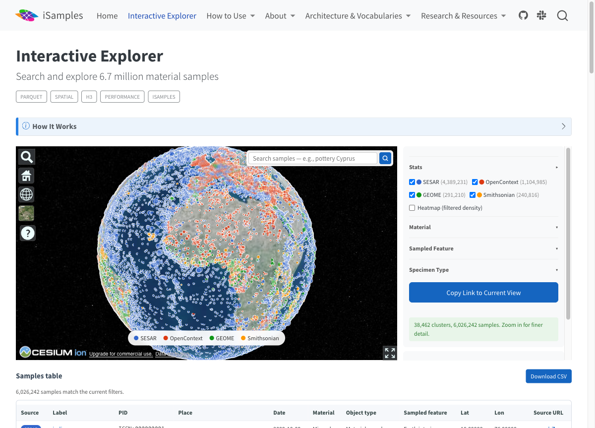
The first thing the globe tells you is where science samples the world — and where it doesn’t. Blue (SESAR) dots trace the oceans: decades of marine cores and dredges. Red (OpenContext) concentrates in the Mediterranean and Near East: archaeological excavation. Green (GEOME) follows biodiversity fieldwork; yellow (Smithsonian) reflects museum collections. Sampling is not uniform — it is a map of scientific attention.

sources = sql(`
  SELECT facet_value AS source, count
  FROM read_parquet('${FACET_SUMMARIES}')
  WHERE facet_type = 'source'
  ORDER BY count DESC`)

Plot.plot({
  marginLeft: 110,
  height: 180,
  x: {label: "located samples", tickFormat: "s"},
  y: {label: null},
  marks: [
    Plot.barX(sources, {y: "source", x: "count",
      fill: d => ({SESAR: "#3366CC", OPENCONTEXT: "#DC3912",
                   GEOME: "#109618", SMITHSONIAN: "#FF9900"}[d.source] || "#666")}),
    Plot.text(sources, {y: "source", x: "count", text: d => d.count.toLocaleString(), dx: 4, textAnchor: "start"})
  ]
})

One honest wrinkle the globe can’t show: these bars total ~6.03 million — the located samples. Roughly 700,000 more records exist in the collection with no usable coordinates: they never appear on the globe or in the viewport table, but a world-scope search still finds them. Counting only what’s visible would overstate the map and understate the archive.

Step 2 — Search that knows concepts

Search “pottery Cyprus” →

1,305 matches; the located top results ring Cyprus as pins.

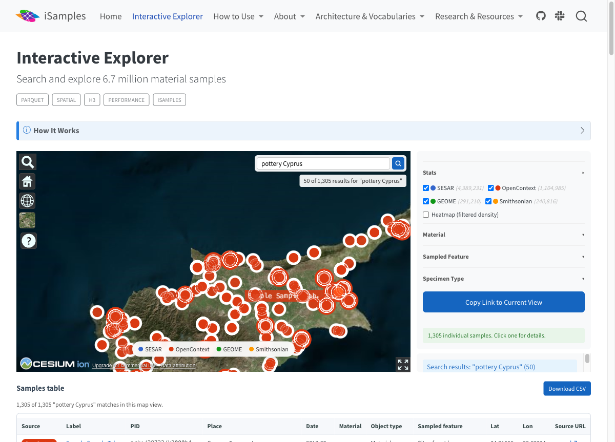
Type pottery Cyprus and 1,305 samples answer, with the top matches pinned on the island. Two things make this more than word-matching. First, the search index folds in vocabulary concepts: a sample tagged with the concept “pottery” matches even if its free text never contains the word. Second, it folds in place names, so “Cyprus” finds samples whose sampling-site place metadata says Cyprus even when their free-text descriptions never mention it. (Both were real user bug reports once — the fixes became the index’s design.)

Search runs on a pre-built sharded index: your query fetches a few small files, not the whole dataset. The classic full-scan search still exists — add &fts=off to the URL to feel the difference.

Step 3 — Two sites, two sciences

Fly to central Anatolia →

The densest region-scale (res4) cell in the collection, centered on the Çatalhöyük region of central Anatolia — shown here in cluster view.

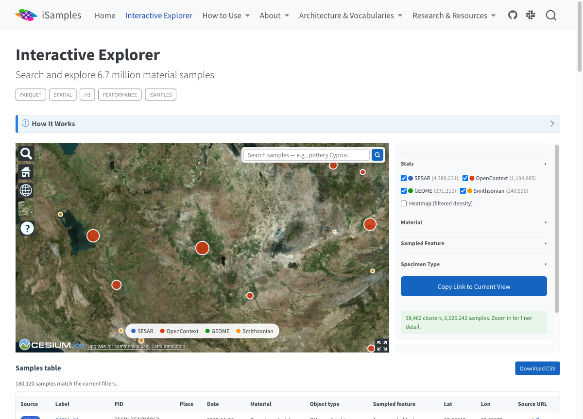
The densest region-scale cell in the whole collection is not over a volcano or a reef — it centers on the countryside around Çatalhöyük, a Neolithic settlement mound in Turkey excavated for decades (the cell aggregates ~150,000 samples from the surrounding region’s digs). Compare Axial Seamount, an undersea volcano off Oregon: basalt collected by submersible. A potsherd from a dig and a basalt from the seafloor carry the same metadata shape — sample, sampling event, site, coordinates, material classification. That shared shape (the iSamples model) is what lets one tool serve both sciences.

dense = sql(`
  SELECT sample_count, center_lat, center_lng, dominant_source
  FROM read_parquet('${H3_RES4}')
  ORDER BY sample_count DESC
  LIMIT 5`)

html`<p><b>The five densest cells on the globe</b> (click to fly there):</p>
<ol>${(await dense).map(d => html`<li>
  <a href="https://isamples.org/explorer.html#v=1&lat=${d.center_lat.toFixed(4)}&lng=${d.center_lng.toFixed(4)}&alt=150000&mode=point" target="_blank">
  ${d.sample_count.toLocaleString()} samples</a> — ${d.dominant_source.toLowerCase()},
  near (${d.center_lat.toFixed(2)}, ${d.center_lng.toFixed(2)})</li>`)}
</ol>`

Step 4 — Slicing by material

Open the Explorer and expand the Material facet →

Check a box — say Mineral — and everything updates together: globe, counts, table. Check two boxes and the counts still hold (that trick, fast multi-filter counting over millions of rows with no server, is most of the Explorer’s hidden machinery). The facet labels are human-readable because a small vocabulary file maps classification URIs to names:

materials = sql(`
  SELECT COALESCE(vl.pref_label, fs.facet_value) AS material, fs.count
  FROM read_parquet('${FACET_SUMMARIES}') fs
  LEFT JOIN read_parquet('${VOCAB_LABELS}') vl ON fs.facet_value = vl.uri AND vl.lang = 'en'
  WHERE fs.facet_type = 'material'
  ORDER BY fs.count DESC
  LIMIT 10`)

Plot.plot({
  marginLeft: 200,
  height: 300,
  x: {label: "located samples", tickFormat: "s"},
  y: {label: null},
  marks: [Plot.barX(materials, {y: "material", x: "count", fill: "#4a7", sort: {y: "-x"}})]
})

Rock and mineral dominate (SESAR’s size shows through), but biogenic and anthropogenic materials are each hundreds of thousands strong — this is genuinely a cross-domain collection, not a geology database with guests.

Step 5 — Density vs identity

Toggle the heatmap → (checkbox in the right panel), and try the 2D map (globe button in the map toolbar → 2D).

Clusters answer “how many, roughly where.” The heatmap answers “where is sampling concentrated” — it makes the Mediterranean glow. Zoomed in, point mode answers “which samples, exactly.” The honest rule of thumb: heatmaps for patterns, points for identity, and never trust a color’s intensity as a count — click and read the number instead.

Step 6 — From view to data-in-hand

Any view’s sample table (below the globe) shows PID, place, date, and a Source URL linking each sample back to its home collection’s record. Download CSV exports up to 50,000 samples matching your current viewport and filters (broader views export the first 50,000). And because the URL carries the whole view state, Copy Link to Current View gives you a citation-grade pointer to this exact slice — paste it in a paper, a class assignment, or an issue report.

Step 7 — Under the hood (and doing this yourself)

There is no server. The Explorer is a static page querying public Parquet files over HTTP range requests with DuckDB-WASM — the code cells on this page use the identical technique against the identical files. To go further:

• EXPLORER_QUERIES.md — plain-English walkthrough of every query the Explorer runs, with copy-paste DuckDB snippets
• CANONICAL.md — which data files are canonical (this page uses only those)
• DATA_PROVENANCE.md — how the derived files are built from the source export (covers the pre-#290/#304 substrate; see its coverage caveat)
• The iSamples Zenodo community — the archived, citable snapshot of the data substrate